


Survival Estimates lymphoma patients
April 28, 2020
Project is based on knowledge of
- Censored Data
- Kaplan-Meier Estimates
1. Import Packages
lifelinesis an open-source library for data analysis.numpyis the fundamental package for scientific computing in python.pandasis what we'll use to manipulate our data.matplotlibis a plotting library.
import lifelines
import numpy as np
import pandas as pd
import matplotlib.pyplot as plt

from lifelines import KaplanMeierFitter as KM
from lifelines.statistics import logrank_test</span>
2. Load the Dataset
from lifelines.datasets import load_lymphoma

def load_data():
    df = load_lymphoma()
    df.loc[:, 'Event'] = df.Censor
    df = df.drop(['Censor'], axis=1)
    return df</span><span id="3504" class="de im gr ef id b db iq ir is it iu io w ip">data = load_data()</span>
first look over your data.
data shape: (80, 3)</span>
The column Time states how long the patient lived before they died or were censored.
The column Event says whether a death was observed or not. Event is 1 if the event is observed (i.e. the patient died) and 0 if data was censored.
Censorship here means that the observation has ended without any observed event. For example, let a patient be in a hospital for 100 days at most. If a patient dies after only 44 days, their event will be recorded as Time = 44 and Event = 1. If a patient walks out after 100 days and dies 3 days later (103 days total), this event is not observed in our process and the corresponding row has Time = 100 and Event = 0. If a patient survives for 25 years after being admitted, their data for are still Time = 100 and Event = 0.
3. Censored Data
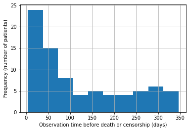
plot a histogram of the survival times to see in general how long cases survived before censorship or events.
data.Time.hist();
plt.xlabel("Observation time before death or censorship (days)");
plt.ylabel("Frequency (number of patients)");</span>

def frac_censored(df):
    """
    Return percent of observations which were censored.

    Args:
        df (dataframe): dataframe which contains column 'Event' which is
                        1 if an event occurred (death)
                        0 if the event did not occur (censored)
    Returns:
        frac_censored (float): fraction of cases which were censored.
    """
    result = 0.0

    result=sum(df['Event']==0) / df.shape[0]

    return result</span> <span id="ce02" class="de im gr ef id b db iq ir is it iu io w ip">print (frac_censored(data))</span><span id="5160" class="de im gr ef id b db iq ir is it iu io w ip">0.325</span>
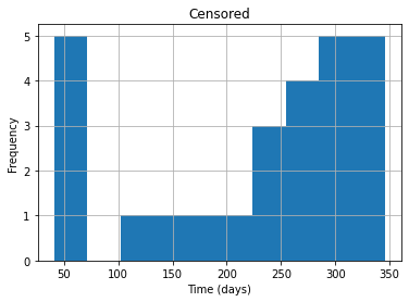
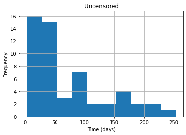
see the distributions of survival times for censored and uncensored examples.
df_censored = data[data.Event == 0]
df_uncensored = data[data.Event == 1]

df_censored.Time.hist()
plt.title("Censored")
plt.xlabel("Time (days)")
plt.ylabel("Frequency")
plt.show()

df_uncensored.Time.hist()
plt.title("Uncensored")
plt.xlabel("Time (days)")
plt.ylabel("Frequency")
plt.show()</span>


4. Survival Estimates
estimate the survival function:
S(t) = P(T > t)
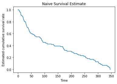
we’ll start with a naive estimator of the above survival function. To estimate this quantity, we’ll divide the number of people who we know lived past time $t$ by the number of people who were not censored before $t$.
Formally, let $i$ = 1, …, $n$ be the cases, and let $t_i$ be the time when $i$ was censored or an event happened. Let $e_i= 1$ if an event was observed for $i$ and 0 otherwise. Then let $X_t = {i : T_i > t}$, and let $M_t = {i : e_i = 1 \text{ or } T_i > t}$. The estimator you will compute will be:
$$ \hat{S}(t) = \frac{|X_t|}{|M_t|} $$
def naive_estimator(t, df):
    """
    Return naive estimate for S(t), the probability
    of surviving past time t. Given by number
    of cases who survived past time t divided by the
    number of cases who weren't censored before time t.

    Args:
        t (int): query time
        df (dataframe): survival data. Has a Time column,
                        which says how long until that case
                        experienced an event or was censored,
                        and an Event column, which is 1 if an event
                        was observed and 0 otherwise.
    Returns:
        S_t (float): estimator for survival function evaluated at t.
    """
    S_t = 0.0

    S_t = (sum(df['Time']>t))/(sum((df['Time']>t)|(df['Event']==1)))

    return S_t</span>
Check for some test cases to see if output is correct. To cross check manually calculate values and crosscheck
print("Test Cases")

sample_df = pd.DataFrame(columns = ["Time", "Event"])
sample_df.Time = [5, 10, 15]
sample_df.Event = [0, 1, 0]
print("Sample dataframe for testing code:")
print(sample_df)
print("\n")

print("Test Case 1: S(3)")
print("Output: {}\n".format(naive_estimator(3, sample_df)))

print("Test Case 2: S(12)")
print("Output: {}\n".format(naive_estimator(12, sample_df)))

print("Test Case 3: S(20)")
print("Output: {}\n".format(naive_estimator(20, sample_df)))

# Test case 4
sample_df = pd.DataFrame({'Time': [5,5,10],
                          'Event': [0,1,0]
                         })
print("Test case 4: S(5)")
print(f"Output: {naive_estimator(5, sample_df)}")</span><span id="65b5" class="de im gr ef id b db iq ir is it iu io w ip">Test Cases
Sample dataframe for testing code:
   Time  Event
0     5      0
1    10      1
2    15      0

Test Case 1: S(3)
Output: 1.0

Test Case 2: S(12)
Output: 0.5

Test Case 3: S(20)
Output: 0.0

Test case 4: S(5)
Output: 0.5</span>
We will plot the naive estimator using the real data up to the maximum time in the dataset.
max_time = data.Time.max()
x = range(0, max_time+1)
y = np.zeros(len(x))
for i, t in enumerate(x):
    y[i] = naive_estimator(t, data)

plt.plot(x, y)
plt.title("Naive Survival Estimate")
plt.xlabel("Time")
plt.ylabel("Estimated cumulative survival rate")
plt.show()</span>

Next let’s compare this with the Kaplan Meier estimate.
Kaplan-Meier estimate:
$$ S(t) = \prod_{t_i \leq t} (1 — \frac{d_i}{n_i}) $$
where $t_i$ are the events observed in the dataset and $d_i$ is the number of deaths at time $t_i$ and $n_i$ is the number of people who we know have survived up to time $t_i$.
def HomemadeKM(df):
    """
    Return KM estimate evaluated at every distinct
    time (event or censored) recorded in the dataset.
    Event times and probabilities should begin with
    time 0 and probability 1.

    Example:

    input:

         Time  Censor
    0     5       0
    1    10       1
    2    15       0

    correct output:

    event_times: [0, 5, 10, 15]
    S: [1.0, 1.0, 0.5, 0.5]

    Args:
        df (dataframe): dataframe which has columns for Time
                          and Event, defined as usual.

    Returns:
        event_times (list of ints): array of unique event times
                                      (begins with 0).
        S (list of floats): array of survival probabilites, so that
                            S[i] = P(T > event_times[i]). This
                            begins with 1.0 (since no one dies at time
                            0).
    """
    # individuals are considered to have survival probability 1
    # at time 0
    event_times = [0]
    p = 1.0
    S = [p]

    # get collection of unique observed event times
    observed_event_times = list(df.Time.unique())

    # sort event times
    observed_event_times = sorted(observed_event_times)

    # iterate through event times
    for t in observed_event_times:

        # compute n_t, number of people who survive to time t
        n_t = sum((df['Time'] >= t))

        # compute d_t, number of people who die at time t
        d_t = sum((df['Event'] == 1) & (df['Time'] == t))

        # update p
        p = ((n_t-d_t)/n_t)*p

        # update S and event_times
        event_times.append(t)
        S.append(p)

    return event_times, S</span><span id="54b2" class="de im gr ef id b db iq ir is it iu io w ip">print("TEST CASES:\n")

print("Test Case 1\n")

print("Test DataFrame:")
sample_df = pd.DataFrame(columns = ["Time", "Event"])
sample_df.Time = [5, 10, 15]
sample_df.Event = [0, 1, 0]
print(sample_df.head())
print("\nOutput:")
x, y = HomemadeKM(sample_df)
print("Event times: {}, Survival Probabilities: {}".format(x, y))

print("\nTest Case 2\n")

print("Test DataFrame:")

sample_df = pd.DataFrame(columns = ["Time", "Event"])
sample_df.loc[:, "Time"] = [2, 15, 12, 10, 20]
sample_df.loc[:, "Event"] = [0, 0, 1, 1, 1]
print(sample_df.head())
print("\nOutput:")
x, y = HomemadeKM(sample_df)
print("Event times: {}, Survival Probabilities: {}".format(x, y))</span><span id="8b24" class="de im gr ef id b db iq ir is it iu io w ip">TEST CASES:

Test Case 1

Test DataFrame:
   Time  Event
0     5      0
1    10      1
2    15      0

Output:
Event times: [0, 5, 10, 15], Survival Probabilities: [1.0, 1.0, 0.5, 0.5]

Test Case 2

Test DataFrame:
   Time  Event
0     2      0
1    15      0
2    12      1
3    10      1
4    20      1

Output:
Event times: [0, 2, 10, 12, 15, 20], Survival Probabilities: [1.0, 1.0, 0.75, 0.5, 0.5, 0.0]</span>
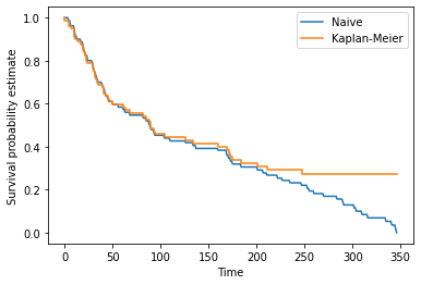
Now let’s plot the two against each other on the data to see the difference.
max_time = data.Time.max()
x = range(0, max_time+1)
y = np.zeros(len(x))
for i, t in enumerate(x):
    y[i] = naive_estimator(t, data)

plt.plot(x, y, label="Naive")

x, y = HomemadeKM(data)
plt.step(x, y, label="Kaplan-Meier")
plt.xlabel("Time")
plt.ylabel("Survival probability estimate")
plt.legend()
plt.show()</span>

5. Subgroup Analysis
We see that along with Time and Censor, we have a column called Stage_group.
- A value of 1 in this column denotes a patient with stage III cancer
- A value of 2 denotes stage IV.
We want to compare the survival functions of these two groups.
This time we’ll use the KaplanMeierFitter class from lifelines. Run the next cell to fit and plot the Kaplan Meier curves for each group.
S1 = data[data.Stage_group == 1]
km1 = KM()
km1.fit(S1.loc[:, 'Time'], event_observed = S1.loc[:, 'Event'], label = 'Stage III')

S2 = data[data.Stage_group == 2]
km2 = KM()
km2.fit(S2.loc[:, "Time"], event_observed = S2.loc[:, 'Event'], label = 'Stage IV')

ax = km1.plot(ci_show=False)
km2.plot(ax = ax, ci_show=False)
plt.xlabel('time')
plt.ylabel('Survival probability estimate')
plt.savefig('two_km_curves', dpi=300)</span>

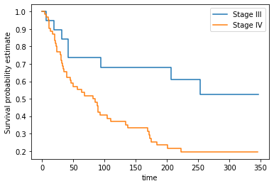
Let’s compare the survival functions at 90, 180, 270, and 360 days
survivals = pd.DataFrame([90, 180, 270, 360], columns = ['time'])
survivals.loc[:, 'Group 1'] = km1.survival_function_at_times(survivals['time']).values
survivals.loc[:, 'Group 2'] = km2.survival_function_at_times(survivals['time']).values</span>
This makes clear the difference in survival between the Stage III and IV cancer groups in the dataset.
5.1 Log-Rank Test
To say whether there is a statistical difference between the survival curves we can run the log-rank test. This test tells us the probability that we could observe this data if the two curves were the same. The derivation of the log-rank test is somewhat complicated, but luckily lifelines has a simple function to compute it.
def logrank_p_value(group_1_data, group_2_data):
    result = logrank_test(group_1_data.Time, group_2_data.Time,
                          group_1_data.Event, group_2_data.Event)
    return result.p_value

logrank_p_value(S1, S2)</span><span id="624f" class="de im gr ef id b db iq ir is it iu io w ip">0.009588929834755544</span>
p value of less than 0.05, which indicates that the difference in the curves is indeed statistically significant.
Credits: Coursera Ai in medicine course
detailed nice font blog in https://kirankamath.netlify.app/blog/survival-estimates-lymphoma-patients/